
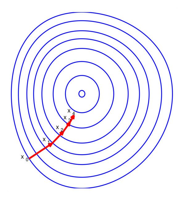
Steepest descent: Data science, Machine Learning, or any Mathematical Optimization related technical interviews encounter the most common question on one of the properties of the method of Steepest Descent. It is also called Gradient Descent method. The successive directions of the steepest descent are normal to one another. They ask for proof or some example to explain this property. In this article, I start with the proof and give a simple example to describe it –
Let  is the starting point of the iterative Steepest descent method to solve
  whose
whose
extremum is  .
.
We update the iterative point as follows:
Next successive point 
The new point is a function of  , the step size.
If  is the function of that decides the new point, the useful value of can be calculated by setting
Note, derivative is w.r.t to ,
![\[\nabla{f(x_1)} = 0.\]](https://i0.wp.com/letsgyan.com/wp-content/ql-cache/quicklatex.com-4fcd871853f06d3889e013080bfb0e54_l3.png?resize=88%2C17&ssl=1 "Rendered by QuickLaTeX.com")
![\[\mbox{or~ } \nabla{f(x_1)} = \frac{{\delta{f(x_1)}}}{\delta{x_1}} \frac{\delta{x_1}}{\delta{t}} = 0.\]](https://i0.wp.com/letsgyan.com/wp-content/ql-cache/quicklatex.com-890898ab04e54f3de2836687bd28ab5b_l3.png?resize=216%2C38&ssl=1 "Rendered by QuickLaTeX.com")
![\[\mbox{or~ } \nabla{f(x1)} = \frac{{\delta{f(x1)}}}{\delta{x1}} \frac{{\delta{(x0 - t \cdot \nabla{f(x0)})}}}{\delta{t}} = 0, \mbox{~here $x_1 = x_0 - t \cdot \nabla{f(x_0)}$}.\]](https://i0.wp.com/letsgyan.com/wp-content/ql-cache/quicklatex.com-b0470e51006b210b581911c3209ad551_l3.png?resize=522%2C35&ssl=1 "Rendered by QuickLaTeX.com")
If we further simplify
![\[\frac{{\delta{f(x_1)}}}{\delta{x_1}}. ( 0 - 1 \cdot \nabla{f(x_0)}) = 0\]](https://i0.wp.com/letsgyan.com/wp-content/ql-cache/quicklatex.com-e36acf4fa9ee5dcee3e0ca9f7d380070_l3.png?resize=200%2C38&ssl=1 "Rendered by QuickLaTeX.com")
Now we have,
![\[\frac{{\delta{f(x_1)}}}{\delta{x_1}} \cdot \nabla{f(x_0)} = 0.\]](https://i0.wp.com/letsgyan.com/wp-content/ql-cache/quicklatex.com-7ff63212e04f8aa9b26cf5674f97b045_l3.png?resize=149%2C38&ssl=1 "Rendered by QuickLaTeX.com")
![\[\mbox{Or~~} \frac{{\delta{f(x_1)}}}{\delta{x_1}} \cdot \frac{{\delta{f(x_0)}}}{\delta{x_0}} = 0.\]](https://i0.wp.com/letsgyan.com/wp-content/ql-cache/quicklatex.com-f32faab696c19a6b8e9970f2def0cb8b_l3.png?resize=179%2C38&ssl=1 "Rendered by QuickLaTeX.com")
From above it looks clear that the product of successive gradients is = 0. Hence from the basic definition of gradient, successive gradients are orthogonal to each other.
Note:  means derivative of
  at point

Understand with one simple example
From example,  is a function of two variables.
Starting point  is given.
Now, gradient of at  is
is
(1) 
According to Steepest Descent rule, new update point
 time the negative of the gradient of at
i.e.,

So,

Note, new point
 is a function of , we call it the step size.
 Function value at new point will also be a function of
,  .
.Now, gradient of
at  ~ w.r.t.~ is
 (2) 
We set
 , it gives us t = 0.2.
 Now new point we have is

From 1 and 2 we have, and 
The dot product of two vectors:
![\[2.6 (\hat{i}) + 6.3 (\hat{j}). 3.484 (\hat{i}) + -0.774 (\hat{j}) =0.\]](https://i0.wp.com/letsgyan.com/wp-content/ql-cache/quicklatex.com-e395b208bd1b1c37369f55a2bdddc7a7_l3.png?resize=290%2C20&ssl=1 "Rendered by QuickLaTeX.com")
Also read Column Generation Method for Cutting Stock Problem